3 minutes
Let’s talk about SGD: Stochastic Gradient Descent
It is well known that the Neural Network model is functioning by cooperation of two major components:
- A “loss function”
- An “optimizer”
The loss function measures the disparity between the the target’s true value and the value the model predicts. There are many kinds of loss function in building the NN model, such as MAE (mean absolute error), MSE(mean-squared error) and Huber loss. I will summarize different usages of them in another post. For now, just understand that the loss function is a guide for finding the correct values of the model’s weights (lower loss is better).
Optimizer is an algorithm that adjusts the weights to minimize the loss. Mathematically, gradient descent was described as following if the model is linear:
$$\begin{align*} \text{repeat}&\text{ until convergence:} \lbrace \newline w &= w - \alpha \frac{\partial J(w,b)}{\partial w} \newline b &= b - \alpha \frac{\partial J(w,b)}{\partial b} \newline \rbrace \end{align*}$$
where, parameters 𝑤 and 𝑏 are updated simultaneously.
The gradient is defined as:
$$ \begin{align} \frac{\partial J(w,b)}{\partial w} &= \frac{1}{m} \sum\limits_{i = 0}^{m-1} (f_{w,b}(x^{(i)}) - y^{(i)})x^{(i)} \newline \frac{\partial J(w,b)}{\partial b} &= \frac{1}{m} \sum\limits_{i = 0}^{m-1} (f_{w,b}(x^{(i)}) - y^{(i)})\ \end{align} $$
 |
|---|
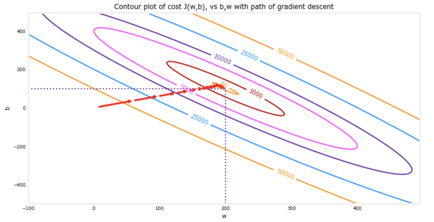
The contour plot above shows the \(loss\)(𝑤,𝑏) over a range of 𝑤 and 𝑏 . Loss levels are represented by the rings. Overlayed red arrows, is the path of gradient descent. Here are some things to note:
- The path makes steady progress toward its goal.
- Initial steps are much larger than the steps near the goal.
Almost all optimization algorithms used in deep learning belong to stochastic gradient descent. When applying it in building Neural Network models, the math part can be directly left to Tensorflow.
Basically, they are iterative algorithms that train a network in steps. One step of training goes like this:
- Sample some training data and run it through the network to make predictions.
- Measure the loss between the predictions and the true values.
- Finally, adjust the weights in a direction that makes the loss smaller.
Then just do this over and over until the loss won’t decrease any further.
 |
|---|
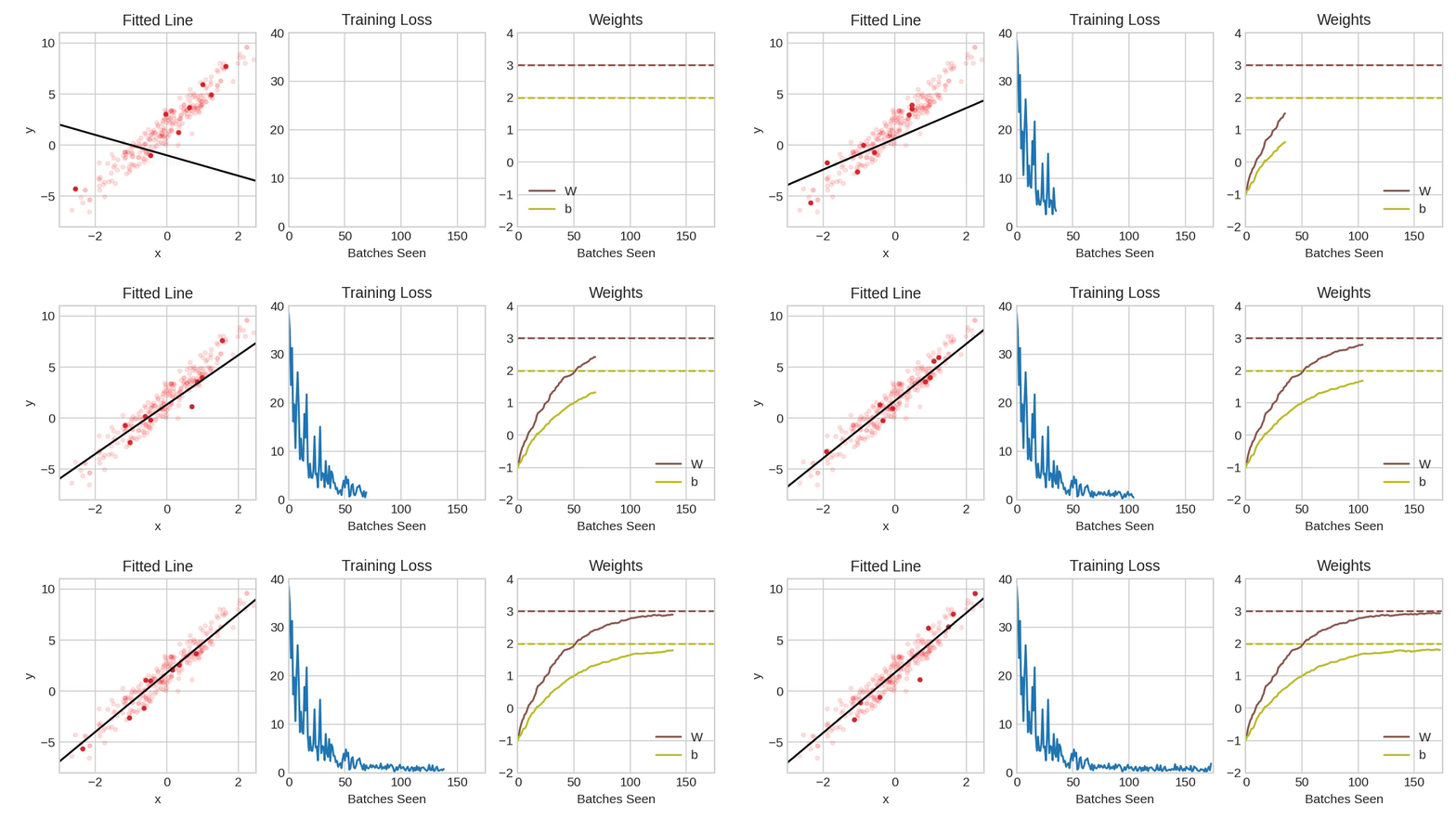
| Training a neural network with Stochastic Gradient Descent.(Source: Kaggle) |
From above animation, the pale red dots depict the entire training set, while the solid red dots are the batches. Every time SGD sees a new batch, it will shift the weights (𝑤 the slope and 𝑏 the y-intercept) toward their correct values on that batch. Batch after batch, the line eventually converges to its best fit. You can see that the loss gets smaller as the weights get closer to their true values.
Btw, each iteration’s sample of training data is called a batch, while a complete round of the training data is called an epoch.
One more thing we need to pay attention is the learning rate α. The larger α is, the faster gradient decent converge. On the other hand, if α is too large, the gradient decent will diverge and never find the right parameters. Therefore, choosing the right α is crucial. However, one SGD algorithm called Adam has an adaptive learning rate that makes it suitable for most problems without any parameter tuning. This characteristics makes it a great general purpose optimizer.
When a model is built through Tensorflow.keras, adding only a few lines of codes will do the job:
model.compile(optimizer="adam", loss="mae",)
Certainly the loss function can be substituted by others, and there are several parameters to tune for Adam, I will cover this topic in another post.